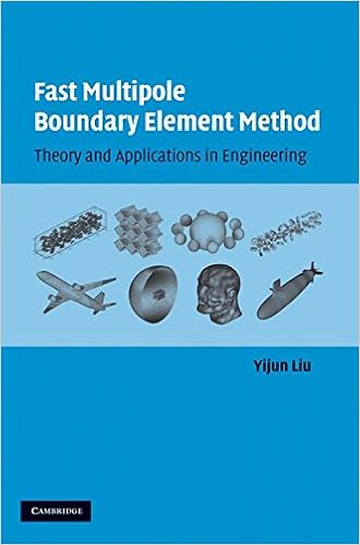
By Yijun Liu
The short multipole technique is among the most crucial algorithms in computing constructed within the twentieth century. besides the short multipole strategy, the boundary aspect technique (BEM) has additionally emerged, as a strong process for modeling large-scale difficulties. BEM versions with thousands of unknowns at the boundary can now be solved on computer desktops utilizing the short multipole BEM. this is often the 1st booklet at the speedy multipole BEM, which brings jointly the classical theories in BEM formulations and the new improvement of the short multipole technique. - and three-d strength, elastostatic, Stokes circulation, and acoustic wave difficulties are coated, supplemented with workout difficulties and computing device resource codes. functions in modeling nanocomposite fabrics, bio-materials, gas cells, acoustic waves, and image-based simulations are tested to teach the possibility of the quick multipole BEM. This publication may help scholars, researchers, and engineers to benefit the BEM and quick multipole process from a unmarried resource.
Read or Download Fast Multipole Boundary Element Method: Theory and Applications in Engineering PDF
Similar applied books
Interactions Between Electromagnetic Fields and Matter. Vieweg Tracts in Pure and Applied Physics
Interactions among Electromagnetic Fields and subject offers with the foundations and techniques which can enlarge electromagnetic fields from very low degrees of signs. This ebook discusses how electromagnetic fields may be produced, amplified, modulated, or rectified from very low degrees to permit those for software in communique structures.

Krylov Subspace Methods: Principles and Analysis
The mathematical conception of Krylov subspace equipment with a spotlight on fixing structures of linear algebraic equations is given an in depth remedy during this principles-based e-book. ranging from the belief of projections, Krylov subspace tools are characterized via their orthogonality and minimisation houses.
This paintings was once compiled with elevated and reviewed contributions from the seventh ECCOMAS Thematic convention on clever buildings and fabrics, that used to be held from three to six June 2015 at Ponta Delgada, Azores, Portugal. The convention supplied a accomplished discussion board for discussing the present cutting-edge within the box in addition to producing notion for destiny principles particularly on a multidisciplinary point.
- Applied Nonlinear Analysis
- Matrix Computations and Semiseparable Matrices: Linear Systems
- Parallel Processing and Applied Mathematics: 7th International Conference, PPAM 2007, Gdansk, Poland, September 9-12, 2007 Revised Selected Papers
- Applied Inverse Problems: Select Contributions from the First Annual Workshop on Inverse Problems
Additional resources for Fast Multipole Boundary Element Method: Theory and Applications in Engineering
Sample text
Constant elements are used for all the examples, and reasonably accurate BEM solutions are obtained. Linear or quadratic elements can be applied to improve the accuracy of the BEM solutions (see problems). 16. A spherical perfect conductor meshed with 4800 elements. 3. 00000 the fast multipole solution techniques to demonstrate the computational efficiencies of the fast multipole BEM for solving large-scale problems. 13 Summary In this chapter, the BIE formulations for solving potential problems are presented.
In the case of using constant elements, we have N = M. 3. Discretization of boundary S using constant elements. where φ j and q j ( j = 1, 2, . . , N) are the nodal values of φ and q, respectively, on element S j for constant elements. 27) Sj where Gi and Fi are the kernels with the source point x placed at node i. 17) for node i: 1 φi = 2 N gi j q j − fˆi j φ j , for i = 1, 2, . . 28) j=1 where the coefficients are given by: gi j = Gi dS, Sj fˆi j = Fi dS, for i, j = 1, 2, . . , N. 1). In matrix form, Eq.
For example, on element Sk (k = 1, 2, 3, . . 33) α=1 2 q(y) = q(ξ ) = α=1 where φ 1 , φ 2 and q1 , q2 are the nodal values of φ and q at local nodes 1 and 2, respectively; ξ is the local (natural) coordinate defined on the element; and N1 (ξ ) and N2 (ξ ) are the linear shape functions given by: N1 (ξ ) = 1 − ξ, N2 (ξ ) = ξ. 34) Placing source point x at node i (i = 1, 2, 3, . . 37) Sk with i = 1, 2, 3, . . , N (number of nodes), k = 1, 2, 3, . . , M (number of elements), and a = 1 and 2 (number of local nodes on each element).